Chap5. Sorting¶

约 378 个字 104 行代码 2 张图片预计阅读时间 3 分钟

本章节介绍排序算法。

5.1 Preliminaries¶

统一接口：void X_Sort(ElementType A[], int N)
只考虑内排（内存能装下）
基于【比较】的排序

5.2 Insertion Sort¶

斗地主摸牌方式排序。

void insertion_sort(ElementType A[], int N)
{
    for(int i=1;i<N;i++)
    {
        ElementType temp=A[i];
        for(int j=i; j>0 && A[j-1]>temp ;j--)
            A[j]=A[j-1];
        A[j]=temp;
    }
}

Worst case: Reverse order, \(T(N)=O(N^{2})\).

Best case: Sorted order, \(T(N)=O(N)\).

5.3 A Lower Bound for Simple Sorting Algorithms¶

\(T(N,I)=O(I+N)\)，其中\(I\)是序列中逆序对的数量。

5.4 Shell Sort¶

定义增量序列\(h_{1}<h_{2}<\cdots,h_{t}\)，\((h_{1}=1)\)

void Shellsort(ElementType A[], int N)
{
    int d;
    for(d=N/2;d>0;d/=2)
    {
        for(int i=d;i<N;i++)
        {
            ElementType temp=A[i];
            for(int j=i;j>=d;j-=d)
            {
                if(temp<A[j-d])
                    A[j]=A[j-d];
                else break;
                A[j]=temp;
            }
        }
    }
}

Worst Case: \(\Theta(N^{2})\).

改进：Hibbard's Increment Sequence，最坏情况为\(\Theta(N^{1.5})\)，平均情况为\(\Theta(N^{1.25})\).

5.5 Heap Sort¶

建堆，随后不断调用DeleteMax/Min。

void heapsort(ElementType A[], int N)
{
    for(int i=N/2;i>=0;i--)
        percdown(A,i,N);
    for(int i=N-1;i>0;i--)
    {
        swap(&A[0],&A[i]);
        percdown(A,0,i);
    }
}

\(T(N)=O(NlogN)\)

实际表现不如使用Sedgewick增量序列的希尔排序。

5.6 Merge Sort¶

5.6.1 Merge¶

Merge是一种合并两个有序序列为一个新的有序序列的操作。

void merge(ElementType A[], ElementType temp[], int left, int right, int rightend)
{
    int leftend=right-1;
    int temppos=left;
    while(left<=leftend && right<rightend)
    {
        if(A[left]<=A[right])
            temp[tempppos++]=A[left++];
        else
            temp[tempppos++]=A[right++];
    }
    while(left<=leftend) temp[temppos++]=A[left++];
    while(right<=rightend) temp[tempppos++]=A[right++];

    for(int i=0;i<rightend-left+1;i++)
        A[i]=temp[i];
}

5.6.2 MergeSort¶

void Msort(ElementType A[], ElementType temp[], int left, int right)
{
    if(left<right)
    {
        int center=(left+right)/2;
        Msort(A, temp, left, center);
        Msort(A, temp, cneter+1, right);
        merge(A, temp, left, center+1, right);
    }
}

5.6.3 Analysis¶

\(T(N)=T(N+NlogN)=T(NlogN)\)

并且需要\(O(N)\)的线性存储空间。

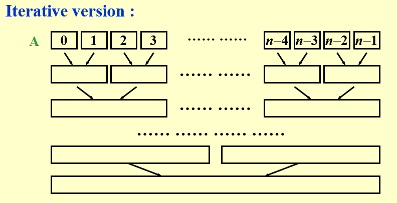
可以改造成迭代版本，每相邻两段做merge操作。

5.7 Quick Sort¶

The fastest known sorting algorithm in practice.

5.7.1 Algorithm¶

void quicksort(ElementType A[], int N)
{
    if(N<2) return ;
    choose pivot;
    Partition S={A[]\pivot} into :
        A1={a|a<=pivot}, A2={a|a>=pivot};
    A=quicksort(A1)+{pivot}+quicksort(A2);
}

Best case: \(T(N)=O(NlogN)\)

The pivot is placed at the right place once and for all. Pivot 第一次排序后就一直在其正确位置上了。

5.7.2 Picking the Pivot¶

Pivot=median(left,center,right)

ElementType median3(ElementType A[], int left, int right)
{
    int center=(left+right)/2;
    if(A[left]>A[center]) swap(&A[left],&A[center]);
    if(A[left]>A[right]) swap(&A[left],&A[right]);
    if(A[center]>A[right]) swap(&A[center],&A[right]);
    /* A[left]<A[center]<A[right] */
    swap(&A[center],&A[right-1]);
    return A[right-1];
}

5.7.3 Implement¶

void quicksort(ElementType A[], int left, int right, int cutoff)
{
    if(cutoff<=right-left)
    {
        int pivot=median3(A,left,right);
        int i=left; int j=right-1;
        while(1)
        {
            while(A[++i]<pivot) {};
            while(A[--j]>pivot) {};
            if(i<j)
                swap(&A[i],&A[j]);
            else break;
        }
        swap(&A[i],&A[right-1]);
        quicksort(A,left,i-1);
        quicksort(A,i+1,right);
    }
    else
        insertion_sort(A+left,right-left+1);
}

5.7.4 Analysis¶

Worst case: \(T(N)=O(N^{2})\)

Best case: \(T(N)=O(NlogN)\)

Average case: \(T(N)=O(NlogN)\)

5.8 A General Lower Bound for Sorting¶

对于基于【比较】的排序算法，最坏时间复杂度一定是\(\Omega(NlogN)\)，不能再小了。

5.9 Sorting Large Structures¶

采用非直接排序：Table sort，对指针排序。

5.10 Bucket Sort and Radix Sort¶

5.10.1 Bucket Sort¶

一分一段表可以种这种方式排序。

不基于【比较】，而是依据数据的范围（要求为有界整数）构建对应的\(N\)个bucket，遇到一个直接放进对应的A[bucket]里面即可。

线性时间即可完成排序。\(T(N)=O(N)\)

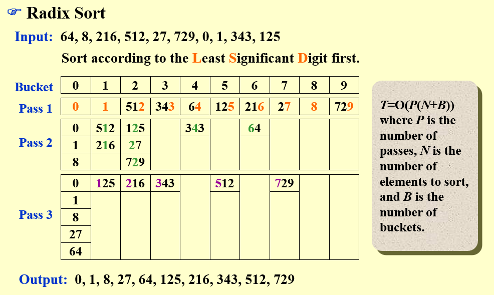
5.10.2 Radix Sort¶

根据数据特定位上的数据分类排序，称为基数排序。

例如LSD排序：先排个位：0~9；再放十位、百位等等，直到都排好。

MSD同理，从最高位开始。